MOS 2010 Excel Expert Beta Exam Information (77-888)

The Excel Expert beta exam is accepting registration now.

The beta exam is free, but you will face more questions than that from actual exam.

The exam content objectives be found from this link:

Just taken the exam today, I think is about 80% tougher than the "specialist" one.
Besides formula building, more steps were needed for each questions to be done.
(In my opinion, this exam do have more advanced topics than that in 2000~2003 experts exam, e.g. array formula)

When preparing for this exam, make sure that you have some experience on those sub-objectives
(i.e. "This objective may include but is not limited to...")
You will meet MOST (almost all) of them in the exam.
Besides, just like all other MS exams, there should have some questions about 2010 new features.

Here are the objectives that "expanded" for a little bit
Sharing and Maintaining Workbooks

•Apply workbook settings, properties, and data options.
This objective may include but is not limited to: setting advanced properties, saving a workbook as a template, and mapping/importing/exporting XML data

•Apply protection and sharing properties to workbooks and worksheets.
◦This objective may include but is not limited to: protecting the current sheet, protecting the workbook structure, restricting permissions, and requiring a password to open a workbook

•Maintain shared workbooks.
◦This objective may include but is not limited to: merging workbooks and setting Track Changes options

Applying Formulas and Functions
•Audit formulas.
◦This objective may include but is not limited to: tracing formula precedents, dependents, and errors, locating invalid data or formulas, and correcting errors in formulas

•Manipulate formula options.◦This objective may include but is not limited to: setting iterative calculation options and enabling or disabling automatic workbook calculation

•Perform data summary tasks.◦This objective may include but is not limited to: using an array formula and using SUMIFS function (Remember the brothers of SUMIFS) 

•Apply functions in formulas.◦This objective may include but is not limited to: finding and correcting errors in functions, applying arrays to functions, and using lookup, Statistical, Date and Time, Financial, Text, and Cube functions
(Common function from each of the above categories)

Presenting Data Visually
•Apply advanced chart features.◦This objective may include but is not limited to: using Trend lines, Dual axes, chart templates, and Sparklines, "Dynamic Chart" (i.e. chart with filtered data)

•Apply data analysis.◦This objective may include but is not limited to: using automated analysis tools and performing What-If analysis (i.e. Scenario/Goal Seek), Data Consolidation

•Apply and manipulate PivotTables.◦This objective may include but is not limited to: manipulating PivotTable data and using the slicer to filter and segment your PivotTable data in multiple layers

•Apply and manipulate PivotCharts.◦This objective may include but is not limited to: creating, manipulating, and analyzing PivotChart data

•Demonstrate how to use the slicer.◦This objective may include but is not limited to: choosing data sets from external data connections ("External" means pivot table that other than currently selected)

Working with Macros and Forms
•Create and manipulate macros.◦This objective may include but is not limited to: running a macro, running a macro when a workbook is opened, running a macro when a button is clicked, recording an action macro, assigning a macro to a command button, creating a custom macro button on the Quick Access Toolbar, and applying modifications to a macro

•Insert and manipulate form controls.◦This objective may include but is not limited to: inserting form controls and setting form controls properties


----
Last Updated at: 2010-12-24

Excel 2010: Where is the "Office button -> Prepare" in Excel 2010?

The Prepare Tab in office button of Excel 2007 has been reorganized completely into Info Tab of File menu in Excel 2010.

If you are going to take MOS 2010 Exam, it is better to take a look at the new locations:

Properties: (The most "hidden" one) Now you can go to advanced properties with fewer click(s).

Inspect Documents

Encrypt Documents, Add a Digital Signature & Mark as Final

The Encrypt Document is the same as Tools->General Options->Password to Open in the Save As dialog box

Run Compatibility Checker:

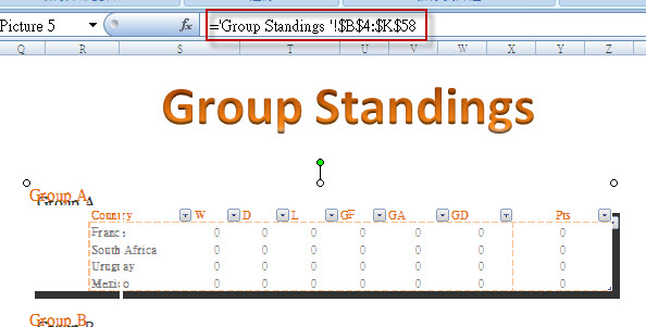
Excel 2007/2010: "World Cup 2010" Excel Template: Dynamic Image

A good template that demonstrated how to use a dynamic image.
World Cup 2010 Excel template
In the "Group Stage" sheet, the content of image on the right side is based "Group Standings" sheet.
There is a formula in the image to redirect content from specified cell location.

MOS 2007 logo changes

Just a very short blog about MCAS (Microsoft Certified Application Specialists)

This month, MCAS title and logo has been changed back to Microsoft Office Specialists

New logo

Old logo

 

Excel: Wired sorting results in Pivot Table and solution

Summary

You may see that the sorting on text column going strange like below.

The Left side is a normal data range. The right side is a pivot table that with source from A1:A7

Possible Cause

The problem has been caused by sorting with "custom list" under PivotTable.

The "Custom List" is used to instruct the Excel the sorting order of a list of items.

An example custom list: "JAN", "FEB", "MAR"

should be sorted as "JAN", "FEB", "MAR", but not alphabetically  "FEB", "JAN", "MAR"

There are two types of "custom List", one is Excel built-in (including Months,Day of weeks...), another type is user defined.

The "Custom List" could be reviewed or adjusted with following location:

Excel 2010:  File->Option->Advanced->Edit Custom Lists (General Section)

Excel 2007: Office button->Excel Options->Popular-> Edit Custom Lists (button)

Excel 2000/XP/2003: Tools->Option->Custom Lists (Tab)

Symptoms

Assume that we feeding a list of 3 alphabet into a pivottable to sort: "AAA","AAB"..."AAZ","ABA"...."ZZZ" 

The "sorted" result from Pivottable would become this:

You could see the list is started with "Months" JAN but not AAA

Resolution and Workaround

Excel 2007/2010

A. To switch off the custom list sorting on pivot table

1. Right Click the PivotTable-> PivotTable Options
2. Totals & Filters-> remove the check box from "Use Custom Lists when sorting"

B. To switch off the individual column custom list ordering

1. Right Click the Field required -> Sort->More Sort Option
2. In the "Sort Options", Make sure "Ascending" or "Decending" selected.
3. Click on the "More Options" Button
4. Remove the checkbox: "Sort automatically every time the report is updated"
5. Select "No Calculation" in first key sort order
6. Press OK twice

Excel 2003

C. To switch off the individual column custom list ordering

1. Right click the Field required, go to Data Menu->Sort
2. Click on Options button, select "normal" in custom sort order
3. Press OK twice

Excel PivotTable Autofilter on data value

When working with pivot table,
you may find the Autofilter feature for data value is disabled from Pivot table.

2010

2003

To take the autofilter for data value, first, select the cell near the header like below image.

After that, go to Data Ribbon(2007/2010)/Menu(2003/XP)->filter again,

you would see that the Autofilter feature is back

2010

2003 

However, beware that the Total value are not affected by the autofilter function.

2010

2003

If showing total value for filter data required, it could be achieved by setting up some helper formulas and then add it to page filter.

For Programmers
If your existing application are accessing the old preview box.
you can still access the old preview mode. It's also not inside the 2010 object model change list:

ActiveWindow.SelectedSheets.PrintPreview 

Formula Recipe:Random order list

To transform a given list of item in random order, the following formula could be used:
RAND - for creating random number
ROW - used with RAND to generate random number
LARGE - To match out the list from ranking.
VLOOKUP - used with LARGE for locate exact position of item

Assume the list of Target is located in column B


Step1: add formula in A2:
=INT(RAND()*1000)+ROW()/10000
the "ROW()/10000" is used to prevent duplicated random number.Even the rand() result is 0, the default ranking would be row number. The 10000 is the possible number of items in the list.

Step 2: add formula in D2:
=LARGE(A$2:A$21,ROW()-1)

To generate sorted list of rank
Step 3: add formula in E2
=VLOOKUP(D2,A$1:B$21,2,FALSE)
Based on the sorted list of rank, look for the sorted list of targets.

Step 4: extend the formula in A2,D2 and E2 to number items by copy and paste

Finish!

Excel 2010: Print Preview Full Screen (Old Print Preview)

For Users

From menu controls, the new print preview mode has completely replaced the old print preview.
The new print preview mode offer a streamlined "quick printing" in one screen:
Selecting printer, number of copies, paper orientation,... All in One

However, convenience control "margin manual tuning" (as below) is missing from the new mode.

Actually, the old print preview is still not removed.
You can add it to the quick access bar, or any ribbon (new ribbon customization feature in Office 2010)

The below steps demonstrate how to release the old print preview (Print Preview Full Screen) method to the quick access bar

Step 1:Click on the more 

Step 2:

Finish, Click this button to launch the old print preview screen:

---

For Programmers

If your existing application are accessing the old preview box.

you can still access the old preview mode. It's also not inside the 2010 object model change list:

ActiveWindow.SelectedSheets.PrintPreview

Microsoft Certified Application Specialist(MCAS) credential change

According to wendyj, the Microsoft Certified Application Specialist (MCAS) will be rebranded to Microsoft Office Specialist (MOS) at June/2010.

It seems that the new brand (MCAS) like MCITP doesn't heard by many employers.
Many of the employer's still only knows about MCSE but not MCITP (We can find it out from the recruit).


Besides, there are far too more MOSs than MCASs in the world.

Anyway, there will have new logos for the MOS.
About the old MCAS certificates or cards with MCAS logo, you may use them for lighting up the BBQ stove. :)

Office 2010 Code (VBA) Compatability Inspector

To check whether existing VBA codes supported by Office 2010 or not,
instead of re-compiling the VBA codes, Microsoft now offering a new inspector for you.

Gray has written a short guide about on how to use the inspector.
If your macros are password protected, remember to unlock it before launching the inspector.

However, this tools is still in beta. I have encountered serveral false alarm about "Range" objects.

As the tools are in beta, you can send any feedback to the development team.
There is also a sweeptakes on bug reporting.

MCAS Practice Test Excel (70-602) Suggested Solutions

(Last Updated 2010-02-28)
Belows are the suggested solution of the practice test.
The steps below is not the only answer.
There may have other ways or even shortcut leading to the same result.

Part I Q1-Q10 Part II Q11-Q20 Part III Q21-Q25

Question 1.

1. Remove the duplicated entry of Vendor Name(Column B) from the range "A3:K159".
Solution:

1. Highlight the range "A3:K159".
2. Data Ribbon > Data Tools Group > Remove Duplicates
3. Make sure that ONLY the box of "Vendor Name" (or Column B) is checked. (Uncheck all others) and then click on OK.

2. Name the cell range "B4:B107": Vendors.

1. Highlight the range "B4:B107".
2. Formulas Ribbon > Defined Name Group > Define name.
3. Enter "Vendor" in the Name box and then click on OK.

MCAS Practice Test Excel (70-602) Q21~25 of 25

(Last Questions Updated: 2010-02-28)

Here is the Third part of the MCAS Excel Practice Test series
For instructions, please refer to the Part I , Part II

---

Question 21

Complete the following THREE tasks:
1.On the current worksheet, insert a chart that compare the products (Column B) with Total Cost Total (Column C), Sales Amount (Column D) and Profit/Loss (Column E) as a clustered cylinder chart (notes: accept all default settings).
2. Move the chart to new worksheet (notes: accept all default settings).
3. Format the chart on the discounts worksheet with the chart style 10.

MCAS Practice Test Excel (70-602) Q11~20 of 25

(Last Questions Updated: 2010-02-28)


Here is the second part of the MCAS Excel Practice Test series
For instructions, please refer to the Part I , next part: Part III

---

Question 11

Complete the following TWO tasks:
1.Insert a function in cell G2 that counts only those customers owned 2 or more cars "G5:G29".
2.Set the sheet tab color as "Orange, Accent 6, Lighter 40%".

MCAS Practice Test Excel (70-602) Q1-10 of 25

(Last Questions Updated: 2010-02-21 Fixed 1st Q/4th Q)
Part II Q11-Q20 Part III Q21-Q25 Solutions

In the following weeks, I will keep posting practice questions/solutions about MCAS.
The questions are inspired from the practice test provided by Arashi (Website in Chinese). Most of the sample data are obtained from SQL Server Adventure works sample database.

---

Instructions
- Each questions consists of 1 to 5 sub-tasks.
- The "Excel format" below is built with editGrid. Those excel could be downloaded for practice. By clicking on the small triangle at the left hand conner of each table, and then click on "Download Excel" option.
- Practice File could also be downloaded with this link
- Column Name / Cell Range are in italic format
- Manual Entries are marked in blue color e.g. Vendors

*Important: the exercises belows by no means copying from actual exam questions, it's just for practice purpose. There is no guarantee on pass even if you finish all the questions below. However, if you know about all of the question, it will be too hard for you to get a low score.

**Welcome for Feedback! please feel free to leave a message at the link in the bottom of this blog.

---

Question 1

Complete the following TWO tasks:
1. Remove the duplicated entry of Vendor Name(Column B) from the range "A3:K159".
2. Name the cell range "B4:B107": Vendors.

Wanna some game with Excel?

Officelabs now offering a game over the actual Excel application. 

The "game" also has a little practice about the "main" new feature of Excel 2010, sparksline.

Your score could also be published to facebook newsfeed.

Step by Step:Excel Watermark (Excel 2010,2007)

Word has a feature on creating warkmark text, such as "Confidential", "Draft",....
However, there no such direct feature in Excel.

The below steps "mimic" the watermark feature in Excel 2007/2010
1. Select the sheet you want to add the watermark
2. Locate Page setup properties

3. Go to the third tab "Header/footer" Click on the custom headaer

4. a)Enter the watermark text you want in the Center Section.

4. b)Highlight the wording and then Click on "A" button to adjust the font size & light color.

 

In this sample, font "Arial" of size 48 has been used for the word "CONFIDENTIAL"

Click OK two times to return to page setup (one time for "Font setting" and one time for "Header")

4. c)If necessary, image could also be added

5. Go to the second tab "Margin".

"Push" the header to the centre of the paper, by adjusting the Header position. For A4 paper, it's 5" roughly.

6. Click OK to finish the setting.

Preview of printout: (Screen from Excel 2010)

Last Updated 2012-APR-13