Excel: Wired sorting results in Pivot Table and solution

Summary

You may see that the sorting on text column going strange like below.

The Left side is a normal data range. The right side is a pivot table that with source from A1:A7

Possible Cause

The problem has been caused by sorting with "custom list" under PivotTable.

The "Custom List" is used to instruct the Excel the sorting order of a list of items.

An example custom list: "JAN", "FEB", "MAR"

should be sorted as "JAN", "FEB", "MAR", but not alphabetically  "FEB", "JAN", "MAR"

There are two types of "custom List", one is Excel built-in (including Months,Day of weeks...), another type is user defined.

The "Custom List" could be reviewed or adjusted with following location:

Excel 2010:  File->Option->Advanced->Edit Custom Lists (General Section)

Excel 2007: Office button->Excel Options->Popular-> Edit Custom Lists (button)

Excel 2000/XP/2003: Tools->Option->Custom Lists (Tab)

Symptoms

Assume that we feeding a list of 3 alphabet into a pivottable to sort: "AAA","AAB"..."AAZ","ABA"...."ZZZ" 

The "sorted" result from Pivottable would become this:

You could see the list is started with "Months" JAN but not AAA

Resolution and Workaround

Excel 2007/2010

A. To switch off the custom list sorting on pivot table

1. Right Click the PivotTable-> PivotTable Options
2. Totals & Filters-> remove the check box from "Use Custom Lists when sorting"

B. To switch off the individual column custom list ordering

1. Right Click the Field required -> Sort->More Sort Option
2. In the "Sort Options", Make sure "Ascending" or "Decending" selected.
3. Click on the "More Options" Button
4. Remove the checkbox: "Sort automatically every time the report is updated"
5. Select "No Calculation" in first key sort order
6. Press OK twice

Excel 2003

C. To switch off the individual column custom list ordering

1. Right click the Field required, go to Data Menu->Sort
2. Click on Options button, select "normal" in custom sort order
3. Press OK twice

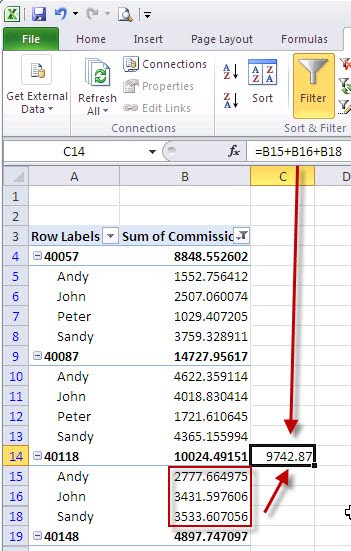
Excel PivotTable Autofilter on data value

When working with pivot table,
you may find the Autofilter feature for data value is disabled from Pivot table.

2010

2003

To take the autofilter for data value, first, select the cell near the header like below image.

After that, go to Data Ribbon(2007/2010)/Menu(2003/XP)->filter again,

you would see that the Autofilter feature is back

2010

2003 

However, beware that the Total value are not affected by the autofilter function.

2010

2003

If showing total value for filter data required, it could be achieved by setting up some helper formulas and then add it to page filter.

For Programmers
If your existing application are accessing the old preview box.
you can still access the old preview mode. It's also not inside the 2010 object model change list:

ActiveWindow.SelectedSheets.PrintPreview 

Excel 2010: Print Preview Full Screen (Old Print Preview)

For Users

From menu controls, the new print preview mode has completely replaced the old print preview.
The new print preview mode offer a streamlined "quick printing" in one screen:
Selecting printer, number of copies, paper orientation,... All in One

However, convenience control "margin manual tuning" (as below) is missing from the new mode.

Actually, the old print preview is still not removed.
You can add it to the quick access bar, or any ribbon (new ribbon customization feature in Office 2010)

The below steps demonstrate how to release the old print preview (Print Preview Full Screen) method to the quick access bar

Step 1:Click on the more 

Step 2:

Finish, Click this button to launch the old print preview screen:

---

For Programmers

If your existing application are accessing the old preview box.

you can still access the old preview mode. It's also not inside the 2010 object model change list:

ActiveWindow.SelectedSheets.PrintPreview

Wanna some game with Excel?

Officelabs now offering a game over the actual Excel application. 

The "game" also has a little practice about the "main" new feature of Excel 2010, sparksline.

Your score could also be published to facebook newsfeed.

Step by Step:Excel Watermark (Excel 2010,2007)

Word has a feature on creating warkmark text, such as "Confidential", "Draft",....
However, there no such direct feature in Excel.

The below steps "mimic" the watermark feature in Excel 2007/2010
1. Select the sheet you want to add the watermark
2. Locate Page setup properties

3. Go to the third tab "Header/footer" Click on the custom headaer

4. a)Enter the watermark text you want in the Center Section.

4. b)Highlight the wording and then Click on "A" button to adjust the font size & light color.

 

In this sample, font "Arial" of size 48 has been used for the word "CONFIDENTIAL"

Click OK two times to return to page setup (one time for "Font setting" and one time for "Header")

4. c)If necessary, image could also be added

5. Go to the second tab "Margin".

"Push" the header to the centre of the paper, by adjusting the Header position. For A4 paper, it's 5" roughly.

6. Click OK to finish the setting.

Preview of printout: (Screen from Excel 2010)

Last Updated 2012-APR-13

Excel:1-minute Tricks Series Vol.1:Format Painter Special feature

Without re-do formatting or re-entry data every time,
"Format Painter" providing a convenient ways on copying formats from one position to others.

Just like copy and paste, select the cells to copy first.
And then, click on the format painter


Notice that the cursor will become brush style


Select the target location/range, done!


I think many of you already know the above...
So what about the "special feature"?

You can also paste the format to multiple locations but without copying multiple times.

Double click the format painter when copy.
Even something has been pasted, the button will not be restored.

To stop the format painter, press "Esc" on keyboard.

This feature also applied to Excel 97 and later on version.

That's all of the first trick!

Excel: 此"列"不同彼"列"

神把人的語言分拆了,但人們只懂使其更複雜...
下面的是真人真事.

與香港客戶對話:

我:就是這個"列"有問題吧?
客:什麼列? 這兩"行"有問題...
我:ok,我幫你檢查一下這"行".

與大陸同事對話:

我:可以幫忙刪去這個值(欄)嗎?
同事:刪去這"列"對吧?
我:不是這"列",是這"欄".
同事:刪去這"列"就行了嗎?
我:不是這"列",是這"欄"!!!!
同事:...就是這"列"吧,不知你"欄"是什麼意.
...

...投降啦.我以後還是用英語啦

相信這個是比較特別的例子
其他的會是功能上,但做成亂的機會比較少:
樞紐表vs透視表,宏 vs 宏集 vs 巨集.

(2010-01-26 後記: 日本語版本跟簡體版一樣,也是"行"+"列")

Excel: Copying formula

In some situation that you may need to edit the formula in batch,
Besides using the replace function, you can use the "formula view"

By pressing "CTRL+`" (Button for ~),
or (Excel before 2007) Tools->Option->View->Windows Option->[Formula]
(Excel 2007) Formula Ribbon-> Formula Auditing->Display formula

You can view and even copy the formula to other application e.g. Notepad/Ultra Editor

MCAS: 77-602 Excel Exam Syllabus breakdown

The Excel 2007 exam syllabus has many changes comparing to the previous exam (2003, 2003 Expert)
The objectives are also became abstracted. The content in 2003 are much detailed to task level.
If you get confused with some 2007 sub-topic.
let's check with the breakdown below. The breakdown is summarized from the official study guide.

1. Creating and Manipulating Data
1.1. Insert data by using AutoFill
- Filling Series
- AutoFill Option on adjacent cell e.g. format
- Custom Fill List
- Copy text/format to adjacent cell
1.2. Ensure data integrity
- Validation
- Remove Duplicate Rows
1.3. Modify cell contents and formats
- Paste special
1.4. Change Worksheet Views
- page layout: Views (e.g. page break view)
- Zoom
- Ribbon Display/Formula bar
- Freeze and split
- Multiple Window
1.5. Manage worksheets
- Hide/Show
- moving and copying



2. Formatting Data and Content
2.1. Format worksheets
-Themes(Apply,Modify,Custom Template)
-Page Layout: Grid lines and heading
-Worksheet Tabs name/Color/Background(WordArts)
2.2. Insert and modify rows and columns
- Insert/Delete, Hide/Show, Height/Width/AutoFit,
- Other Formating e.g. TextWrap/Align/Orientation
2.3. Format cells and cell content
- Standard Format(curreny/text/date...) , Custom Format
- Hyperlinks
- Merged Cell
- Formating(Font,border)
- Cell styles
2.4. Format data as a table
- Include Table Style,Total Row


3. Creating and Modifying Formulas
3.1. Reference data in formulas
- absolute reference, 3D reference
- name: define, manage
3.2. Summarize data using a formula
- sum/count/counta(Count empty)/average/min/max
3.3. Summarize data using subtotals
- subtotal (outlining)
3.4. Conditionally summarize data by using a formula
- averageif,countif,sumif,averageifs,countifs,sumifs
3.5. Look up data by using a formula
- vlookup/hlookup
3.6. Use conditional logic in a formula
- if,and,or,not,iferror
3.7. Format or modify text by using formulas
- lower,proper,upper,
- replace substitute
- text to columns feature
3.8. Display and print formulas
- display formula (ctrl+`)

4. Presenting Data Visually
4.1. Create and format charts
plot chart-chart type, switch column
moving to another sheet
sizing, format ->size
4.2. Modify charts
editing data
range selector
chart element
chart title/format,axes/legend, data labels,gridlines
4.3. Apply conditional formatting
4.4. Insert and modify illustrations
- insert/replace
- insert in footer
- smart arts
- sharps/replace/add text/modify
4.5. Outline data
4.6. Sort and filter data

5. Collaborating and Securing Data
5.1. Manage changes to workbooks
- change tracking
- comment
5.2. Protect and share workbooks
- password protect workbooks
- workbook/worksheet protection
- workbook sharing
5.3. Prepare workbooks for distribution
- workbook properties
- document inspectors
- restrict permission
- digital signatures
- finalizing
5.4. Save workbooks
- file format
- compatibiltiy checker
5.5. Set print options for printing data, worksheets, and workbooks
- page break
- page setup
- header and footer

Sub topics removed from the final syllabus (May be merged with others)
5.6. Filter data by using AutoFilter
5.7. Filter and sort data by using conditional formatting
5.8. Filter and sort data by using cell attributes


However, It's recommended to practice some feature not appeared but related too, for example, pivot table.

Excel 2007 Multi Language Interface comparison (Menu) 介面多語言對比 (菜單編)

EXCEL 2007 多語言菜單對比 (繁中/簡中/English/日本語),
方便要處理兩岸三地不同用戶語言的支援人員朋友 (包括我自己...)

HOME





INSERT





PAGE LAYOUT




FORMULA





DATA





REVIEW





VIEW





DEVELOPER