Excel 2007/2010: "World Cup 2010" Excel Template: Dynamic Image

A good template that demonstrated how to use a dynamic image.
World Cup 2010 Excel template
In the "Group Stage" sheet, the content of image on the right side is based "Group Standings" sheet.
There is a formula in the image to redirect content from specified cell location.

Excel: Wired sorting results in Pivot Table and solution

Summary

You may see that the sorting on text column going strange like below.

The Left side is a normal data range. The right side is a pivot table that with source from A1:A7

Possible Cause

The problem has been caused by sorting with "custom list" under PivotTable.

The "Custom List" is used to instruct the Excel the sorting order of a list of items.

An example custom list: "JAN", "FEB", "MAR"

should be sorted as "JAN", "FEB", "MAR", but not alphabetically  "FEB", "JAN", "MAR"

There are two types of "custom List", one is Excel built-in (including Months,Day of weeks...), another type is user defined.

The "Custom List" could be reviewed or adjusted with following location:

Excel 2010:  File->Option->Advanced->Edit Custom Lists (General Section)

Excel 2007: Office button->Excel Options->Popular-> Edit Custom Lists (button)

Excel 2000/XP/2003: Tools->Option->Custom Lists (Tab)

Symptoms

Assume that we feeding a list of 3 alphabet into a pivottable to sort: "AAA","AAB"..."AAZ","ABA"...."ZZZ" 

The "sorted" result from Pivottable would become this:

You could see the list is started with "Months" JAN but not AAA

Resolution and Workaround

Excel 2007/2010

A. To switch off the custom list sorting on pivot table

1. Right Click the PivotTable-> PivotTable Options
2. Totals & Filters-> remove the check box from "Use Custom Lists when sorting"

B. To switch off the individual column custom list ordering

1. Right Click the Field required -> Sort->More Sort Option
2. In the "Sort Options", Make sure "Ascending" or "Decending" selected.
3. Click on the "More Options" Button
4. Remove the checkbox: "Sort automatically every time the report is updated"
5. Select "No Calculation" in first key sort order
6. Press OK twice

Excel 2003

C. To switch off the individual column custom list ordering

1. Right click the Field required, go to Data Menu->Sort
2. Click on Options button, select "normal" in custom sort order
3. Press OK twice

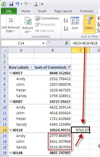
Excel PivotTable Autofilter on data value

When working with pivot table,
you may find the Autofilter feature for data value is disabled from Pivot table.

2010

2003

To take the autofilter for data value, first, select the cell near the header like below image.

After that, go to Data Ribbon(2007/2010)/Menu(2003/XP)->filter again,

you would see that the Autofilter feature is back

2010

2003 

However, beware that the Total value are not affected by the autofilter function.

2010

2003

If showing total value for filter data required, it could be achieved by setting up some helper formulas and then add it to page filter.

For Programmers
If your existing application are accessing the old preview box.
you can still access the old preview mode. It's also not inside the 2010 object model change list:

ActiveWindow.SelectedSheets.PrintPreview 

Formula Recipe:Random order list

To transform a given list of item in random order, the following formula could be used:
RAND - for creating random number
ROW - used with RAND to generate random number
LARGE - To match out the list from ranking.
VLOOKUP - used with LARGE for locate exact position of item

Assume the list of Target is located in column B


Step1: add formula in A2:
=INT(RAND()*1000)+ROW()/10000
the "ROW()/10000" is used to prevent duplicated random number.Even the rand() result is 0, the default ranking would be row number. The 10000 is the possible number of items in the list.

Step 2: add formula in D2:
=LARGE(A$2:A$21,ROW()-1)

To generate sorted list of rank
Step 3: add formula in E2
=VLOOKUP(D2,A$1:B$21,2,FALSE)
Based on the sorted list of rank, look for the sorted list of targets.

Step 4: extend the formula in A2,D2 and E2 to number items by copy and paste

Finish!

MCAS Practice Test Excel (70-602) Suggested Solutions

(Last Updated 2010-02-28)
Belows are the suggested solution of the practice test.
The steps below is not the only answer.
There may have other ways or even shortcut leading to the same result.

Part I Q1-Q10 Part II Q11-Q20 Part III Q21-Q25

Question 1.

1. Remove the duplicated entry of Vendor Name(Column B) from the range "A3:K159".
Solution:

1. Highlight the range "A3:K159".
2. Data Ribbon > Data Tools Group > Remove Duplicates
3. Make sure that ONLY the box of "Vendor Name" (or Column B) is checked. (Uncheck all others) and then click on OK.

2. Name the cell range "B4:B107": Vendors.

1. Highlight the range "B4:B107".
2. Formulas Ribbon > Defined Name Group > Define name.
3. Enter "Vendor" in the Name box and then click on OK.

MCAS Practice Test Excel (70-602) Q21~25 of 25

(Last Questions Updated: 2010-02-28)

Here is the Third part of the MCAS Excel Practice Test series
For instructions, please refer to the Part I , Part II

---

Question 21

Complete the following THREE tasks:
1.On the current worksheet, insert a chart that compare the products (Column B) with Total Cost Total (Column C), Sales Amount (Column D) and Profit/Loss (Column E) as a clustered cylinder chart (notes: accept all default settings).
2. Move the chart to new worksheet (notes: accept all default settings).
3. Format the chart on the discounts worksheet with the chart style 10.

MCAS Practice Test Excel (70-602) Q11~20 of 25

(Last Questions Updated: 2010-02-28)


Here is the second part of the MCAS Excel Practice Test series
For instructions, please refer to the Part I , next part: Part III

---

Question 11

Complete the following TWO tasks:
1.Insert a function in cell G2 that counts only those customers owned 2 or more cars "G5:G29".
2.Set the sheet tab color as "Orange, Accent 6, Lighter 40%".

MCAS Practice Test Excel (70-602) Q1-10 of 25

(Last Questions Updated: 2010-02-21 Fixed 1st Q/4th Q)
Part II Q11-Q20 Part III Q21-Q25 Solutions

In the following weeks, I will keep posting practice questions/solutions about MCAS.
The questions are inspired from the practice test provided by Arashi (Website in Chinese). Most of the sample data are obtained from SQL Server Adventure works sample database.

---

Instructions
- Each questions consists of 1 to 5 sub-tasks.
- The "Excel format" below is built with editGrid. Those excel could be downloaded for practice. By clicking on the small triangle at the left hand conner of each table, and then click on "Download Excel" option.
- Practice File could also be downloaded with this link
- Column Name / Cell Range are in italic format
- Manual Entries are marked in blue color e.g. Vendors

*Important: the exercises belows by no means copying from actual exam questions, it's just for practice purpose. There is no guarantee on pass even if you finish all the questions below. However, if you know about all of the question, it will be too hard for you to get a low score.

**Welcome for Feedback! please feel free to leave a message at the link in the bottom of this blog.

---

Question 1

Complete the following TWO tasks:
1. Remove the duplicated entry of Vendor Name(Column B) from the range "A3:K159".
2. Name the cell range "B4:B107": Vendors.

Wanna some game with Excel?

Officelabs now offering a game over the actual Excel application. 

The "game" also has a little practice about the "main" new feature of Excel 2010, sparksline.

Your score could also be published to facebook newsfeed.

Step by Step:Excel Watermark (Excel 2010,2007)

Word has a feature on creating warkmark text, such as "Confidential", "Draft",....
However, there no such direct feature in Excel.

The below steps "mimic" the watermark feature in Excel 2007/2010
1. Select the sheet you want to add the watermark
2. Locate Page setup properties

3. Go to the third tab "Header/footer" Click on the custom headaer

4. a)Enter the watermark text you want in the Center Section.

4. b)Highlight the wording and then Click on "A" button to adjust the font size & light color.

 

In this sample, font "Arial" of size 48 has been used for the word "CONFIDENTIAL"

Click OK two times to return to page setup (one time for "Font setting" and one time for "Header")

4. c)If necessary, image could also be added

5. Go to the second tab "Margin".

"Push" the header to the centre of the paper, by adjusting the Header position. For A4 paper, it's 5" roughly.

6. Click OK to finish the setting.

Preview of printout: (Screen from Excel 2010)

Last Updated 2012-APR-13

Excel:1-minute Tricks Series Vol.1:Format Painter Special feature

Without re-do formatting or re-entry data every time,
"Format Painter" providing a convenient ways on copying formats from one position to others.

Just like copy and paste, select the cells to copy first.
And then, click on the format painter


Notice that the cursor will become brush style


Select the target location/range, done!


I think many of you already know the above...
So what about the "special feature"?

You can also paste the format to multiple locations but without copying multiple times.

Double click the format painter when copy.
Even something has been pasted, the button will not be restored.

To stop the format painter, press "Esc" on keyboard.

This feature also applied to Excel 97 and later on version.

That's all of the first trick!

Office 2010 Beta Activation issue

When there is a problem on activiting the office beta:
"The setup controller has encountered a problem during install. Please review the log files for further information on the error."


Try the steps below:
1. Launch the setup program "setup.exe" under this location
C:\Program Files\Common Files\microsoft shared\OFFICE14\Office Setup Controller

2. Select "Enter a product key"


3. Click on continue

4. Wait the excel for re-deploy.... and click OK

5. Launch Excel again (or any Office program you like). This option is now back.


6. Wait again for the activiton. Click close when reaching this screen.


7. Restart the Excel. Finish!

Excel VBA Stub: Rearranging Sheets

Codes for re-ordering worksheet
subSplitAndHideSheets: split and hide sheets that not appeared on list: strSheetsAll

------------------

Sub subLaunch
    dim strSheetsAll as string
    strSheetsAll = "Sheet1;Sheet3;Sheet2"
    call subSplitAndHideSheets(strSheetsAll)
end sub


Sub subSplitAndHideSheets(wbCurr As Workbook, strSheetsAll as string)

    Dim strSheets() As String
    Dim strSheetsSD
    Dim intSheetsCounter As Integer
    Dim intSheetsCount As Integer
    Dim intCurrSheet As Integer


    If strSheetsAll = "" Then
        Exit Sub 'Exit sub if not given
    End If

    Set strSheetSD = CreateObject("Scripting.Dictionary")

    strSheets = Split(strSheetsAll, ";")
    intCurrSheet = 1
    intSheetsCount = UBound(strSheets)
    For intSheetsCounter = 0 To UBound(strSheets)
        If funcChkSheetExist(wbCurr, strSheets(intSheetsCounter)) Then
            strSheetSD.Add (UCase(strSheets(intSheetsCounter))), Nothing
            wbCurr.Sheets(strSheets(intSheetsCounter)).Move before:=Sheets(intCurrSheet)
            intCurrSheet = intCurrSheet + 1
        End If
    Next

    intSheetsCount = wbCurr.Worksheets.Count
    If intSheetsCount <= 1 Then
        Exit Sub
    End If
    For intSheetsCounter = 1 To wbCurr.Worksheets.Count
        If wbCurr.Sheets(intSheetsCounter).Visible = xlSheetVisible Then
        'set as hidden: if Sheet not exist in given string array and name is  not parameters
            If Not strSheetSD.exists(UCase(wbCurr.Sheets(intSheetsCounter).Name)) And _
                UCase(wbCurr.Sheets(intSheetsCounter).Name) <> STRSHEETNAME_PARAMETERS Then
                wbCurr.Sheets(intSheetsCounter).Visible = xlSheetHidden
            End If
        End If
    Next
End Sub

Function funcChkSheetExist(wbCurr As Workbook, strSheet As String)
On Error GoTo errHandling
    Dim tmpVal
    tmpVal = wbCurr.Sheets(strSheet).Range("A1")
    funcChkSheetExist = True
    Exit Function
errHandling:
    funcChkSheetExist = False
End Function

Excel: 此"列"不同彼"列"

神把人的語言分拆了,但人們只懂使其更複雜...
下面的是真人真事.

與香港客戶對話:

我:就是這個"列"有問題吧?
客:什麼列? 這兩"行"有問題...
我:ok,我幫你檢查一下這"行".

與大陸同事對話:

我:可以幫忙刪去這個值(欄)嗎?
同事:刪去這"列"對吧?
我:不是這"列",是這"欄".
同事:刪去這"列"就行了嗎?
我:不是這"列",是這"欄"!!!!
同事:...就是這"列"吧,不知你"欄"是什麼意.
...

...投降啦.我以後還是用英語啦

相信這個是比較特別的例子
其他的會是功能上,但做成亂的機會比較少:
樞紐表vs透視表,宏 vs 宏集 vs 巨集.

(2010-01-26 後記: 日本語版本跟簡體版一樣,也是"行"+"列")

Excel 2010 SSAS Cube Sets.

Following up with SSAS features in Excel 2010
Besides creating sets contain only dimension members or calculated members,
you can them both in the same set:



The magic of the sets could be respected to the new "calculatedmember" property in the connection object:

ActiveWorkbook.connections("...").OLEDBConnection.CalculatedMembers.Add Name:="[Set1]", Formula:= "{....}"

What's New in Excel 2010 (Web Resources)

0.General
Official free ebook on Office 2010 features:
First look in Microsoft Office 2010

1. SSAS Cube Related:

Frederik Vandeputte's Blog
Measures:
Running Total (Year To End),
Displaying Single Measure Multiple times
Dimensions
Interactive Filter (Instance selection on typing)
Dynamic Sets (A user friendly approach :-) )
Create Set base Rows Items
Write Backs

Chris Webb Blog
Dynamic Sets
Sets Creation with UI

2. How to show everything with sparklines

Excel Team
- Sparklines as LINE
- Formats: Low / High
- "sparklines are in an Excel table you can add another row of data and the sparkline group would grow and add another sparkline to the table"

Excel Team
- Sparklines as column
- Formats: Negative Points and Styles

Excel Team (1)
Excel Team (2)
-Sparklines as winloss
- Sparkines axis and Reference Line

Excel Team
- Line Up Points

3. Conditional Formatting
Excel Team
- Icon set now customizable
- "Exception handling" in icon set, e.g. negative value

Excel Team
- Proportional Value Bar
- Negative value Bar
- Formating Border/Fills

4. Charting
Excel Team
- Interactivity: Fields button (selection of range and "drilldown" easily)
- Double click objects to format (am... is it so important?)
- Data points: limit of data points extended.

5. Security
Excel Team
Should be something related to this one...


Excel Team
-Protected view for VBA, in control of file access.

General
Overview from Microsoft

Some screenshots in pre-"technical preview"

Excel:SSAS:Locale Reference 語言設定參考

SSAS/EXCEL語言設定參考孖寶 SSAS/EXCEL Translation reference

1.setting up connection
http://www.extremeexperts.com/sql/Tips/ExcelDiffLocale.aspx
2.Locale code
http://www.krafft.com/scripts/deluxe-calendar/lcid_chart.htm

中文有關設定 Chinese related settings:
繁中: 1028 (TAIWAN)
簡中: 2052 (PRC)
香港地區(3076),澳門地區(5724),最後如果沒在SSAS指定,會resolve成1028(即繁中)
詳看msdn

Where to set excel "default" locale for SSAS connection

Control panel->
regional and language option->
"standards and format" section (UPPER section):
select the region
("location" section setting is NOT related)

SSAS Translation: Enterprise vs Standard
標準版只支援維度內容.
standard version support only translation of content in dimension.

metadata translation的意思是維度名稱,cube部件的名字等等...

Excel: Copying formula

In some situation that you may need to edit the formula in batch,
Besides using the replace function, you can use the "formula view"

By pressing "CTRL+`" (Button for ~),
or (Excel before 2007) Tools->Option->View->Windows Option->[Formula]
(Excel 2007) Formula Ribbon-> Formula Auditing->Display formula

You can view and even copy the formula to other application e.g. Notepad/Ultra Editor

MCAS: 77-602 Excel Exam Content List (From Microsoft Official Courseware)

Following up on Post about MCAS Excel MOC:

I'm going to a some more description or links on each topics.
This post will be the index of it.
However, this will be a long long long project...

Section 1. Excel Essentials
Starting Excel.
Working in the Excel Window.
Using the On-Screen Tools.
Using the Office Button.
Changing Excel’s View.
Splitting a Window.
Opening a New Window.
Working with an Existing Workbook.
Opening an Existing Workbook.
Navigating a Worksheet.
Entering Data in a Worksheet.
Selecting, Editing, and Deleting a Cell’s
Quick-Printing a Worksheet.
Saving an Edited Workbook.
Closing a Workbook.

Section 2. Creating and Editing a Workbook.
Creating a Workbook.
Starting a Sales Report from Scratch.
Populating a Worksheet with Data.
Entering Labels.
Entering Dates.
Entering Values.
Filling a Series with AutoFill.
Cutting, Copying, and Pasting Data.
Copying a Data Series with the Mouse.
Moving a Data Series with the Mouse.
Copying and Pasting Data.
Cutting and Pasting Data.
Editing a Workbook’s Properties.
Setting Basic Properties.
Assigning Keywords to a Document.
Printing a Worksheet.
Setting the Print Area.
Using Print Preview.
Choosing a Printer.
Setting Other Printing Options.
Saving a Workbook for the First Time.
Saving a Workbook under a Different Name.
Saving a Workbook for use in a Previous Version of Excel.
Choosing a Different File Format.

Section 3. Formatting Cells and Ranges.
Inserting and Deleting Cells.
Adding a New Cell to a Worksheet.
Deleting a Cell from a Worksheet.
Manually Formatting Cell
Selecting Cells and Ranges.
Aligning a Cell’s
Choosing Fonts and Font Sizes.
Applying Special Character Attributes.
Changing Font Color.
Filling Cells with Color.
Applying Number Formats.
Wrapping Text in a Cell.
Merging and Splitting Cells.
Placing Borders around a Cell.
Copying Cell Formatting with the Format Painter.
Formatting Cells with Styles.
Applying a Cell Style.
Modifying a Cell Style.
Working with Hyperlinked Data.
Placing a Hyperlink in a Cell.
Removing a Hyperlink.
Applying Conditional Formatting to Cells.
Using the Rule Manager to Apply Conditional Formats.
Allowing Multiple Conditional Formatting Rules to be True.
Applying Specific Conditional Formats.
Clearing a Cell’s Formatting.

Section 4. Worksheet Formatting.
Working with Rows and Columns.
Inserting or Deleting a Row or Column.
Modifying Row Height or Column Width.
Formatting an Entire Row or Column.
Hiding and Unhiding a Row or Column.
Using Themes.
Choosing a Theme for a Worksheet.
Customizing a Theme.
Modifying a Worksheet’s On-Screen Appearance.
Formatting a Worksheet’s Background.
Changing the Color of a Worksheet’s Tab.
Viewing and Printing a Worksheet’s Gridlines.
Viewing and Printing Column and Row Headings.
Inserting Headers and Footers.
Adding Page Numbers to a Worksheet.
Inserting a Built-In Header or Footer.
Adding Content to a Header or Footer.
Page Layout.
Adding and Moving a Page Break.
Setting Margins.
Setting a Worksheet’s Orientation on the Page.
Scaling a Worksheet to Fit on a Printed Page.

Section 5. Managing Worksheets.
Organizing Worksheets.
Copying a Worksheet.
Rearranging the Worksheets in a Workbook.
Renaming a Worksheet.
Hiding and Unhiding a Worksheet.
Inserting a New Worksheet into a Workbook.
Deleting a Worksheet from a Workbook.
Finding and Replacing Data.
Locating Data with the Find Command.
Replacing Data with the Replace Command.
Navigating a Worksheet with the Go To Command.

Section 6. Working With Data.
Ensuring Your Data’s Integrity.
Restricting Cell Entries to Certain Data Types.
Allowing Only Specific Values to Be Entered in Cells.
Removing Duplicate Cells, Rows, or Columns from a Worksheet.
Sorting Data.
Sorting Data on a Single Criterion.
Sorting Data on Multiple Criteria.
Sorting Data by Using Conditional Formatting.
Sorting Data By Using Cell Attributes.
Filtering Data.
Using AutoFilter.
Creating a Custom AutoFilter.
Filtering Data by Using Conditional Formatting.
Filtering Data by Using Cell Attributes.
Subtotaling Data.
Grouping and Ungrouping Data for Subtotaling.
Subtotaling Data in a List.
Setting Up Data in Table Format.
Formatting a Table with a Quick Style.
Inserting a Row for Totals in a Table.
Add and Remove Rows or Columns in a Table.

Section 7. Using Basic Formulas and Functions.
Building Basic Formulas.
Creating a Formula That Performs Addition.
Creating a Formula That Performs Subtraction.
Creating a Formula The Performs Multiplication.
Creating a Formula That Performs Division.
Workplace Ready (Starting a Worksheet from a Template, with focus on built-in formulas?).
Using Cell References in Formulas.
Using Relative Cell References in a Formula.
Using Absolute Cell References in a Formula.
Referring to Data in Another Worksheet.
Referring to Data in Another Workbook.
Using Cell Ranges in Formulas.
Naming a Range.
Changing a Range’s Size.
Keeping Track of Ranges.
Creating a Formula That Operates on a Named Range.
Summarizing Data with Functions.
Using SUM.
Using COUNT.
Using COUNTA.
Using AVERAGE.
Using MIN.
Using MAX.
Using Formulas to Create Subtotals.
Selecting Ranges for Subtotaling.
Modifying a Range in a Subtotal.
Building Formulas to Subtotal and Total.
Controlling the Appearance of Formulas.
Displaying Formulas on the Screen.
Printing Formulas.

Section 8. Using More Advanced Formulas.
Using Formulas to Apply Conditional Formatting.
Using SUMIF.
Using SUMIFS.
Using COUNTIF.
Using COUNTIFS.
Using AVERAGEIF.
Using AVERAGEIFS.
Using Formulas to Look Up Data in a Workbook.
Using VLOOKUP.
Using HLOOKUP.
Adding Conditional Logic Functions to Formulas.
Using IF.
Using AND.
Using OR.
Using NOT.
Using IFERROR.
Using Formulas to Format Text.
Using PROPER.
Using UPPER.
Using LOWER.
Using Formulas to Modify Text.
Using SUBSTITUTE.
Using a Formula to Convert Text to Columns.

Section 9. Creating Charts from Your Data.
Building Charts.
Selecting Data to Include in a Chart.
Choosing the Right Chart for Your Data.
Creating a Bar Chart.
Formatting a Chart with a Quick Style.
Manually Formatting the Parts of a Chart.
Changing the Chart’s Fill Color or Pattern.
Changing the Chart’s Border Line.
Formatting the Data Series.
Modifying the Chart’s Legend.
Modifying a Chart.
Adding Elements to a Chart.
Deleting Elements from a Chart.
Moving a Chart.
Resizing a Chart.
Choosing a Different Chart Type.

Section 10. Adding Pictures and Shapes to a Worksheet.
Inserting Pictures.
Inserting a Picture from a File.
Inserting a Clip Art Picture.
Using SmartArt Graphics.
Adding Shapes.
Drawing Lines.
Inserting Basic Shapes.
Drawing a Block Arrow.
Creating a Flowchart.
Copying or Moving a Graphic.
Formatting Graphics.
Resizing a Graphic.
Rotating a Graphic.
Resetting a Picture to Its Original State.

Section 11. Securing and Sharing Documents.
Securing Your Work before Sharing It with Others.
Protecting a Workbook or Worksheet.
Setting Access Permissions to a Workbook.
Allowing Multiple Users to Edit a Workbook Simultaneously.
Marking a Document as Final.
Digitally Signing a Workbook.
Using the Document Inspector.
Distributing a Workbook by E-Mail.
Tracking Changes to a Workbook.
Turning Change-Tracking On and Off.
Inserting Tracked Changes.
Deleting Your Changes.
Accepting Changes from Another User.
Rejecting Changes from Another User.
Setting Track Change Options.
Adding Comments to a Workbook.
Inserting a Comment.
Viewing Comments.
Editing a Comment.
Deleting a Comment.
Viewing Comments from Another User.

MCAS: 77-602 Excel Exam Syllabus breakdown

The Excel 2007 exam syllabus has many changes comparing to the previous exam (2003, 2003 Expert)
The objectives are also became abstracted. The content in 2003 are much detailed to task level.
If you get confused with some 2007 sub-topic.
let's check with the breakdown below. The breakdown is summarized from the official study guide.

1. Creating and Manipulating Data
1.1. Insert data by using AutoFill
- Filling Series
- AutoFill Option on adjacent cell e.g. format
- Custom Fill List
- Copy text/format to adjacent cell
1.2. Ensure data integrity
- Validation
- Remove Duplicate Rows
1.3. Modify cell contents and formats
- Paste special
1.4. Change Worksheet Views
- page layout: Views (e.g. page break view)
- Zoom
- Ribbon Display/Formula bar
- Freeze and split
- Multiple Window
1.5. Manage worksheets
- Hide/Show
- moving and copying



2. Formatting Data and Content
2.1. Format worksheets
-Themes(Apply,Modify,Custom Template)
-Page Layout: Grid lines and heading
-Worksheet Tabs name/Color/Background(WordArts)
2.2. Insert and modify rows and columns
- Insert/Delete, Hide/Show, Height/Width/AutoFit,
- Other Formating e.g. TextWrap/Align/Orientation
2.3. Format cells and cell content
- Standard Format(curreny/text/date...) , Custom Format
- Hyperlinks
- Merged Cell
- Formating(Font,border)
- Cell styles
2.4. Format data as a table
- Include Table Style,Total Row


3. Creating and Modifying Formulas
3.1. Reference data in formulas
- absolute reference, 3D reference
- name: define, manage
3.2. Summarize data using a formula
- sum/count/counta(Count empty)/average/min/max
3.3. Summarize data using subtotals
- subtotal (outlining)
3.4. Conditionally summarize data by using a formula
- averageif,countif,sumif,averageifs,countifs,sumifs
3.5. Look up data by using a formula
- vlookup/hlookup
3.6. Use conditional logic in a formula
- if,and,or,not,iferror
3.7. Format or modify text by using formulas
- lower,proper,upper,
- replace substitute
- text to columns feature
3.8. Display and print formulas
- display formula (ctrl+`)

4. Presenting Data Visually
4.1. Create and format charts
plot chart-chart type, switch column
moving to another sheet
sizing, format ->size
4.2. Modify charts
editing data
range selector
chart element
chart title/format,axes/legend, data labels,gridlines
4.3. Apply conditional formatting
4.4. Insert and modify illustrations
- insert/replace
- insert in footer
- smart arts
- sharps/replace/add text/modify
4.5. Outline data
4.6. Sort and filter data

5. Collaborating and Securing Data
5.1. Manage changes to workbooks
- change tracking
- comment
5.2. Protect and share workbooks
- password protect workbooks
- workbook/worksheet protection
- workbook sharing
5.3. Prepare workbooks for distribution
- workbook properties
- document inspectors
- restrict permission
- digital signatures
- finalizing
5.4. Save workbooks
- file format
- compatibiltiy checker
5.5. Set print options for printing data, worksheets, and workbooks
- page break
- page setup
- header and footer

Sub topics removed from the final syllabus (May be merged with others)
5.6. Filter data by using AutoFilter
5.7. Filter and sort data by using conditional formatting
5.8. Filter and sort data by using cell attributes


However, It's recommended to practice some feature not appeared but related too, for example, pivot table.